We would love to know how you use the Constant Velocity Car in Your Labs! Share your thoughts and ideas in the comments section below. You never know who you might inspire!

INTRODUCTION

The Framework for K-12 Science Education states that one of the principal goals of science education is to “cultivate students’ scientific habits of mind, develop their capability to engage in scientific inquiry, and teach them how to reason in a scientific context.” (National Research Council, 2012, p.41). As science teachers, we want to engage our students in the process of science, not just expose them to scientific knowledge. We want to give our students opportunities to explore concepts and ideas, and we want students to play an active role in developing and communicating those concepts. We want students to view themselves as active participants in the learning process, not just passive recipients of scientific facts.

After trying different inquiry-based teaching methods throughout my career, I chose to adopt much of the teaching practices associated with the Modeling method (Wells et al., 1995; Jackson et al., 2008). Using the Modeling method gives students regular experiences with the process of science and practice with reasoning within a scientific context. Modeling Instruction is student-centered and gives students many opportunities to “learn by doing: they construct and deploy models of the real world and test their ability to predict new phenomena.”

The following article describes a physics lab that can be used at the start of the year. This lab involves students in developing a procedure, data collection, data analysis, and collaborative discussion. This type of lab activity allows students to experience the process of science while also building a correct scientific understanding of the world around them.

PRE-LAB DISCUSSION:

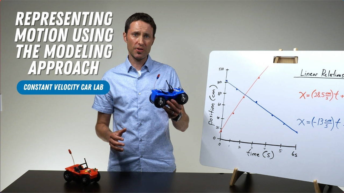
At the start of the year in physics, students need to learn different ways to represent the motion of objects. The motion of objects can be represented using graphs, algebraic equations, diagrams, and verbal descriptions. An easy way to introduce students to some of the different representations of motion is to have them investigate the motion of a battery-operated toy car that moves at a constant speed. These “constant velocity cars” can be purchased from Arbor Scientific. Through this lab experience, students will develop a definition of velocity, learn how to interpret position versus time graphs, and develop an equation that relates an object’s position, time, and velocity at uniform speeds.

Remember, the goal is to have students play an active role in each part of the investigation, but rarely do students come to your classroom already knowing how this is done. This is your opportunity to guide them through the investigative process, inviting them in along the way.

To begin this lab, start by demonstrating the motion of the toy car and ask the students what they observe. Record students’ observations on the board. Try to encourage students to share all of their observations even if those observations are irrelevant to the eventual investigation. There are no wrong answers here. Students may mention that the car’s antenna swings back and forth, or the light on the antenna flashes while it is moving. Both of these observations are irrelevant to the motion of the car’s center of mass but include these observations on the board since you want to encourage student participation. Ultimately, you want the class to recognize that the car is moving at a constant speed in a straight line.

Next, ask the students to identify what can be directly measured about the toy car. Also, list these on the board. For each direct measurement ask the students to identify what measuring tool they would use and what the unit of measure would be. For example, the distance could be measured using a meterstick and the unit of measure would be inches or centimeters. Students often want to measure the speed of the car, but when asked what they would use to directly measure the car’s speed, they mention using a meterstick and stopwatch. A meter stick and stopwatch would be used to directly measure distance and time, not speed. Since speed is not a quantity that can be directly measured, it is left off the list. Common measurements that students identify include the distance traveled by the car, the time it takes to travel a given distance, the car’s weight, the car’s length, and the number of wheel rotations.

Finally, ask students what pairs of measurements they think are possibly related and write these on the board. As a class, the students will investigate the relationship between one of the pairs of variables listed on the board. If a student mentions that they think the distance the car travels and the number of wheel rotations are related, ask them how they think they are related: “As the distance traveled increases, how do you think that affects the number of wheel rotations? Would you expect the number of wheel rotations to increase or decrease? These types of questions help students think qualitatively about how the identified variables might be related. To reach the desired conclusions from the lab experience you need to continue to ask students for possible pairs of related variables until they mention “time” and “distance”. Communicate that ALL of the listed pairs of variables would lead to interesting experiments, but for this lab experience, we will focus on how distance is related to time.

LAB PROCEDURE and DATA COLLECTION:

Now that you have identified a pair of measurable variables which are related, you can write the purpose on the board: “to determine the relationship between the distance the car moves and the time it takes to travel that distance for a car moving at a uniform velocity”.

This is where you can help guide students through a procedure for collecting the needed data. To determine the relationship between any two measured variables, the students will need to collect a variety of different distance and time measurements. This is another place you can invite students into the investigative process. Ask students how this can be done.

While discussing how “distance” can be measured using a meterstick or metric measuring tape, ask students what the numbers on the measuring device represent. Do the numbers represent the distance traveled or something else? Through discussing a couple of examples it should be clear that the meterstick is measuring the “position” of the object, the location of the car relative to some zero point or “origin” on a number line. For example, if a car starts at the 20 cm marking on the measuring tape and moves to the 70 cm marking, the car has traveled a distance of 50 cm. The markings on the measuring tape must then be directly measuring something other than distance traveled. The measuring tape ONLY measures distance traveled if the car starts at the 0 cm mark and moves in the direction of the positive numbers. The car’s location or “position” is what is being directly measured using the measuring tape or meter stick, NOT the distance traveled.

With this in mind, the purpose statement should be rewritten: “to determine the relationship between the position and time of a car moving at a constant speed.”

By the end of the class discussion about how the data will be collected, the students should agree on a method which either measures the time it takes to reach certain specific positions or the position of the car at specific times. The students will need to mark the zero position on the floor before collecting data and decide if the front or the back of the car will represent the car’s position along the measuring tape. A common method for collecting data is to use a dry erase marker to mark the position of the car every 1 second as it moves along the floor. It takes some practice to make a mark at each time interval, so encourage students to try again if they are not confident with their initial markings. A metronome can be used to help time the marks if needed by having it played over a speaker for all students to hear, or encourage lab groups to use a cell phone with headphones for the student marking the car’s position.

A few basic guidelines when determining the type of relationship between two variables is to get a wide range of at least 6 to 8 different values for each variable. Also, during the conclusion discussion, it is beneficial for lab groups to have different-looking data. For this lab, have students use different speed cars, start at different initial positions, and move in different directions. It is helpful to pre-assign these guidelines to each lab group. See the examples below.

Note: You can make the constant velocity cars move slower by replacing one of the two C-cell batteries with a spacer made out of a dead C-cell battery or a wooden dowel wrapped in aluminum foil. I find it helpful to make similarly colored cars move at the same speed. For example, I make the red cars go fast with two C-cells and the blue cars go slow with one battery and one spacer.

DATA ANALYSIS:

To analyze the collected position and time data, have the students graph their data by placing the position values on the y-axis and the time values on the x-axis. Show students how they can write an equation from their graph showing the algebraic relationship between the position and time for their car.

Any linear relationship can be written in the form of y = mx+b, but you want your student’s equations to include the specific variables and values from the graph of their specific data. The following steps can be used to guide students in writing their linear equations from their graphed data.

Step 1: Write the general slope-intercept form of a line: y=mx+b
Step 2: Replace “y” and “x” in the general equation with symbols that represent the variables graphed on each axis. In this lab the letter “x” is used to represent the position, and “t” is used to represent time.
Step 3: Replace “m” and “b” with the numerical values and units of measure for the graph’s slope and y-intercept found using a linear fit of the graph.

Example: The slope of a student’s linear graph is +11cm/s and the y-intercept is 20cm.

Step 1: y = mx+b
Step 2: x = mt + b
Step 3: x = (11cm/s)t + 20cm

Ask each lab group to discuss the shape of their graph and the significance or meaning of both the slope and y-intercept of their graph and equation. These questions will be the main focus of the collaborative discussion when students share their results with the rest of the class.

CONCLUSION DISCUSSION:

To facilitate a whole-class conversation about the relationship between position and time for objects moving at constant speeds, have each lab group record their graph and resulting equation on a large whiteboard. Reasonably priced whiteboards can be purchased from Arbor Scientific.

Have the class circle up so that everyone can clearly see the graphs and equations on each whiteboard. Remember that your goal is to help facilitate a conversation that allows your students to make connections and draw conclusions from the graphs and equations. Within this conclusion discussion, we want students to connect features of their graphs and equations with the motion of the cars used in the experiment.

Start by asking the students to identify any similarities or differences in the graphs or equations. If you give groups different speed cars, starting positions, and directions of motion; then the students will be able to identify similar graphical shapes but different graph steepness or slope values and different y-intercept values.

Now you can ask what led to different or similar slope and y-intercept values. Why were some slopes positive and other slopes negative? The discussion surrounding these questions should lead students to the conclusion that the slope represents both the speed of the car, how many centimeters the car travels each and every second, and the direction the car is moving. A positive slope indicates the car is moving away from the zero position, and a negative slope indicates the car is moving toward the zero position. The students should also conclude that the y-intercept on the position versus time graph is the starting or initial position of the car.

After the class reaches a consensus about the meaning of the slope and y-intercept of the position versus time graphs, use various lab group’s whiteboards to quiz them. Point to a lab group’s whiteboard and see if other groups can identify whether the graph and equation shown represent a “fast” or “slow” car, motion in the positive or negative direction, and the given starting position. Make sure to ask students what specifically about the graph or equation shows the relative speed, direction, and starting position of the car. Do this with several different whiteboards until it is clear that the students can connect features of their graphs and equations with the motion of the car which was used in the experiment.

Each group’s graph and equation only describe how the position of their car is related to time. Now, with a consensus about the meaning of the slope and y-intercept, you can define “velocity” and show students how to write the general equation for all the cars. Remind students that they concluded the slope represents both the speed of the car and its direction of motion. This is the definition of “velocity”: an object’s speed and direction. Also, remind the students that they concluded that the y-intercept of each graph and equation represents the initial position of the car. Simply replace the numbers of the slope and y-intercept with symbols that represent the meaning of each to get the final general equation.

Example Student Equation: x = (11cm/s)t + 20cm

Final General Equation: x = vt + x0

x = position
v = velocity
t = time
x0 = initial position

This general equation not only describes how position and time are related for all of the cars used in the experiments, but it can also be used to make predictions about the motion of these cars or any other object which moves in a straight line at a constant speed. The graphs, linear equations, and verbal descriptions of the car’s motion are all ways to represent the car’s motion and can be used to make predictions about other objects which move in similar ways.

To hear a more detailed explanation of the conclusion discussion you can visit my YouTube channel “Debbink Physics” and search for the video titled “Toy Car Lab (Conclusion Discussion)”. If you are interested in learning more about these types of guided inquiry labs visit www.modelinginstruction.org.

Happy investigating!

Aaron Debbink

We would love to know how you use the Constant Velocity Car in Your Labs! Share your thoughts and ideas in the comments section below. You never know who you might inspire!

REFERENCES

National Research Council. (2012). A Framework for K-12 Science Education: Practices, Crosscutting Concepts, and Core Ideas. Washington, DC: The National Academies Press. https://doi.org/10.17226/13165.

Wells, M., Hestenes, D., & Swackhamer, G. (1995) A modeling method for high school physics instruction. American Journal of Physics, 63, 606 http://modeling.asu.edu/R&E/ModelingMethod-Physics_1995.pdf