INTRODUCTION

Note: This article is written for high school and introductory college level physics and will outline a lab experience that can be used to introduce the thin-lens equation.

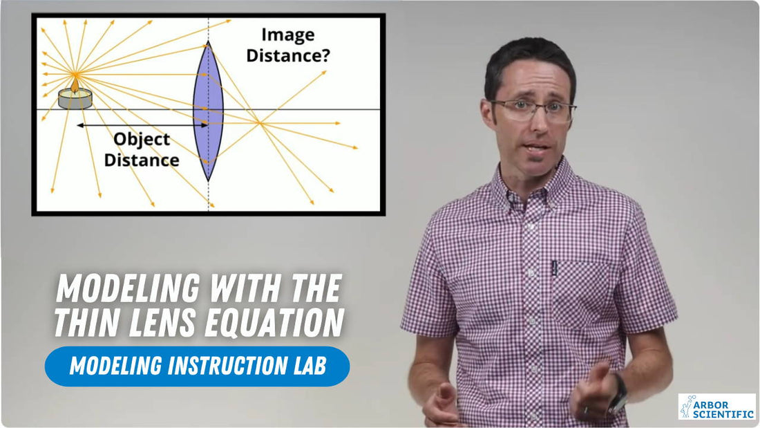
Any introduction to light and optics involves giving students an understanding of basic image formation, and how mirrors and lenses can manipulate light to produce images of objects both on a screen and in the mind of an observer. At the high school and college levels, students must have both a qualitative and quantitative understanding of basic image formation. For example, if an object is placed in front of a converging lens at a specific distance, what kind of image will be formed, and how far away from the lens can the focused image be found? These questions can be answered qualitatively with ray diagrams and quantitatively using what’s known as the “thin lens” equation.

In this article, I will walk you through an introductory physics lab that allows students to develop a model for the relationship between the distance an object is placed from a lens and the distance a focused image will be formed from the lens. This guided investigation will allow students to develop the “thin lens” equation from their experimental data. The “thin lens” equation states that the inverse of the object distance plus the inverse of the image distance is equal to the inverse of the lens’s focal point.

The following equipment is needed for the pre-lab discussion and each lab group.

• (1) Introductory Optical System (Optical Bench)
• (2) From the "Meter Stick 6 pack"

PRE-LAB DISCUSSION

Before starting this lab, students need to be familiar with drawing ray diagrams for both converging and diverging lenses. This understanding is necessary for the pre-lab discussion.

At the start of the pre-lab discussion, show students a variety of ray diagrams, and remind the students how ray diagrams can be used to predict the type and location of a focused image. A scaled ray diagram would allow quantitatively accurate predictions about where a focused image would form, but it would be convenient to have an algebraic equation for this type of determination.

Ask students what variables affect where an image is formed. Based on their understanding of ray diagrams, students should list things such as the type of lens, the distance the object is placed from the lens, and the lens’s focal point distance.

The Introductory Optical System is a great tool which can be used to further investigate how these variables quantitatively affect a focused image’s location.

Briefly show students the LED object and the viewing screen from the Introductory Optical System. Discuss how each LED from the LED object is streaming light in all directions. When the screen is placed very close to the LED object, you can see a small circle of light that strikes the viewing screen from each LED light source. As the viewing screen is moved farther away, the light from each LED is spread out more and creates a larger circle on the viewing screen. The image which forms on the viewing screen is not in focus because the light coming from each part of the LED object is overlapping, and eventually the light that falls on the viewing screen no longer looks like the letter “F” from the LED object.

In order for a focused image to be created on the viewing screen, the light that is spreading out from each LED, must be brought back together again to a common point. Ask students what kind lens brings light rays together, or can focus light rays to a common point. Students will quickly recognize that this can be done with a converging lens. Use one of the converging lenses from the Introductory Optical System to create a focused image of the LED object on the viewing screen. Briefly show that for the given lens, when the distance of the LED object is changed relative to the lens’s location, the distance of the focused image will also change.

Now students are ready to discuss how this apparatus can be used to investigate how the object distance and lens’s focal length quantitatively affect the location of the real image formed on a screen. Tell students that each lab group will be given a converging lens in order to determine the relationship between the distance a real image is formed by a converging lens and the distance the object is from the lens. Now you can help guide students through a procedure for collecting the needed data.

DATA COLLECTION

To determine the relationship between the distance a real image is formed by a converging lens and the distance the object is from the lens, the students will need to collect a variety of different object distances and image distances. Remind students that this can only be done for “real images” that can be produced on the viewing screen. “Virtual images” only appear in the mind of an observer and are more difficult to locate in order to measure the image distance. If you are interested in learning how to experimentally measure the image distance of a virtual image, see the Instructional Guide included with the Introductory Optical System.

Ask students what scenarios will produce real images with a converging lens. Based on their experience with ray diagrams the student should realize that a real image will form ONLY when the object is farther away from the lens than the focal point distance. This means the students will first need to determine the focal length of their converging lens so they can place the object at distances greater than this measurement.

Ask students how they can experimentally determine the focal length of their lens. To help guide them in this discussion, ask students what type of light rays will cross at a converging lens’s focal point. The students will know that all light rays traveling parallel with the principal axis will travel through the lens’s focal point after passing through the lens. Students can use a parallel ray light box or a distant light source like the sun to estimate their lens’s focal length. If they are using the sun to estimate the focal length, guide them through a short discussion showing how light from a distant light source can be approximated as parallel light rays when they pass through a lens at a great distance.

SAFETY NOTE: Remind students they should NEVER attempt to look at the Sun directly or through the converging lens. The students can use a sheet of paper to determine how far away the Sun’s light rays will be focused to a point from the lens. The distance the paper is from the lens is the lens's approximate focal length.

Once students have their experimentally measured focal length, the students can place their LED object at distances greater than this value. These object distances will produce a focused, real image on the viewing screen, and the screen’s distance from the lens will be the “image distance”.

To introduce some variability in the collected data, give half of the lab groups the 100mm focal length converging lens, and the other half the 200mm focal length lens. This variability in the focal length will help the students reach conclusions about their graphs and equations during the conclusion discussion.

Remind students that they should collect a wide range of values, using small and large object distances. This means placing the LED object close to the focal length distance and very far from the lens. Tell students they may need to use a larger surface, like a whiteboard, to locate the real image distance, if the image is far away from the lens. They may also want to use a second meter stick to measure the larger object and image distances.

DATA ANALYSIS

To analyze the collected object distance and image distance data, have students graph their data by placing the image distance values on the y-axis and the object distance values on the x-axis.

Students should find the graphed data will appear to be hyperbolic. Sometimes when students look at their original graph, the trend appears linear with a negative slope. This will typically happen if the students do NOT collect a wide range of object distance values. Upon closer inspection, there is usually a slight upward curve to the data, but the students are not convinced it is nonlinear. Have students go back and collect additional data points where the object distance is close to the focal length. The additional data points should help convince them the original graph is nonlinear.

In order to write the algebraic equation for the relationship between the object distance and the image distance, the students will first need to “linearize” or “re-express” their nonlinear graph. In my class, this is a skill that was introduced in a previous lab. To hear a more detailed explanation of re-expressing or linearizing a nonlinear relationship, check out one of my previous videos from the CoolStuff Blog. The video is titled “Forces and Motion”, and the relevant discussion about linearization starts around 7 minutes into the video.

For this set of experimental data, the graphical relationship is not one that students have seen before. The students will start by using the two most common ways to linearize or “re-express” a hyperbolic graph. This is done by graphing the image distance as a function of either the inverse of the object distance, or the inverse of the object distance squared. Neither option will produce a linear graph. Suggest that the students also try simultaneously modifying the y-axis variable, by taking its inverse or inverse squared. After some more experimentation, students will find a linear graph when they plot the inverse of the image distance as a function of the inverse of the object distance.

If necessary, remind students how they can write an equation from their linearized graph showing the algebraic relationship between the object distance and the image distance.

Any linear relationship can be written in the form of y = mx + b, but you want your students’ equations to include the specific variables and values from the graph of their specific data. The following steps can be used to guide students in writing their linear equations from their graphed data. When students first learn to write an equation from a linear fit, it is helpful for them to write out each of the three steps.

For step number one, write the general slope-intercept form of a line: y = mx + b

For step number two, replace “y” and “x” in the general equation with symbols that represent the variables graphed on each axis. In this expression “1/do” is used to represent the inverse of the object distance, and “1/di” is used to represent the inverse of the image distance.

For step number three, replace “m” and “b” with the numerical values and units of measure for the graph’s slope and y-intercept found using a linear fit of the linearized graph.

Example: The slope of a student’s linear graph is -1.04 cm/cm and the y-intercept is 0.104 1/cm.

Step 1: y = (m)x + b
Step 2: 1/di = (m)1/do + b
Step 3: 1/di = (-1.04 cm/cm)1/do + 0.104 1/cm

Before the students circle up to share the analysis of their results, ask each lab group to discuss the shape of their original graph and the significance or meaning of both the slope and the y-intercept of their linearized graph and equation.

CONCLUSION DISCUSSION

To facilitate a whole-class conversation about the relationship between the object distance and the image distance, have each lab group record their graph and resulting equation on a large whiteboard. Below is an example of what one lab group’s whiteboard would look like. The whiteboard should include the original graph of the collected data, the linearized graph, and the algebraic equation showing the relationship between the two tested variables. Students should make sure to label each axis on both graphs and to include the value and units of measure for both the slope and y-intercept in their equation.

Have the class circle up so that everyone can clearly see the graphs and equations on each whiteboard. Remember that your goal is to help facilitate a conversation that allows your students to make connections and draw conclusions from the graphs and equations.

Start by asking students to compare the graphs and equations on the whiteboards and identify any similarities or differences they see. For this lab, students will have similar graph shapes and slope values, but different y-intercept values. Once the similarities and differences are identified, the rest of the conclusion discussion should focus on what the shape of the graph suggests about the relationship between variables, the meaning of the slope, and the significance of the y-intercept.

Meaning of Slope:

When students look at the slope of the linearized graphs and equations, they should all find values around negative one. If students measured their distances in units of centimeters, they should find that the slope has units of centimeters divided by centimeters, which is just unitless. This suggests that the slope represents either a unitless coefficient, like the coefficient of friction, or the slope represents a ratio of two constants with the same units. In my class this is the third time they have seen a slope value around one, and in both previous cases it was a unitless coefficient that simply showed equality between two ratios. In this case, the students are ready to accept that the slope is simply negative one and does not represent some other variable in the equation.

Meaning of Y-intercept:

When the students look at the values of the y-intercepts they will have small positive values with units of one divided by centimeters. The students are not aware of this at this point, but the groups using lenses with the same focal point will have similar y-intercept values.

Usually the first question is whether the y-intercept is significant. As an initial test, I tell my students that the y-intercept is insignificant if it is less than five percent of the maximum y-value from their linear graph. If this is the case, the y-intercept of the linear fit could reasonably be explained as a result of measurement error and can be considered zero. For this lab, the linearized graph has a negative slope, so the y-intercept for every group is greater than their largest y-value. The y-intercept is more than one hundred percent of the largest y-value. Clearly the y-intercept is significant and must be explained.

Start by reminding students the y-intercept of their linearized graph is one value and must represent something that stayed constant throughout their entire experiment. This constant thing must explain why groups got different y-intercept values, but had the same units: inverse centimeters. Discuss each shared idea to help students decide if this is the meaning of the y-intercept.

You could start by reminding students that the units of a measured value are a good clue to determining what kind of measurement it represents. For example, if the units of a value were seconds, the value must represent a time; if the units of a value was miles divided by hours, the value must represent a speed or velocity. For this lab, the units of one divided by centimeters suggests that the y-intercept must represent one divided by some constant length measurement. Ask students if there was any length measurement related to their experimental setup that did not change throughout the entire experiment. It doesn’t take long for students to suggest that the focal length of their lens was constant. Ask students how the constant focal length of their lens is related to their y-intercept value. The students will quickly determine that the inverse of their focal length is very close to the value of the y-intercept on their linearized graph. This also explains why some of the lab groups had different y-intercepts, because they used lenses with different focal lengths. So the consensus meaning of the y-intercept is that it represents the inverse of the lens’s focal length.

After the students reach a consensus about the meaning of the slope and the y-intercept, you can write the general equation on the board. This general equation now shows the algebraic relationship between the object distance and image distance for any converging lens. It turns out that this equation also works for diverging lenses, and both concave and convex mirrors.

If you are interested in learning more about these types of guided inquiry labs used in the modeling method of instruction visit www.modelinginstruction.org.

Happy investigating!

Aaron Debbink